Table of Contents
- Prerequisites
- Step 1: Setting Up the Environment
- Step 2: Run Jupyter Notebook
- Step 3: Import Required Libraries
- Step 4: Load and Display the Image
- Step 5: Convert the Image to Grayscale
- Step 6: Apply Gaussian Blur
- Step 7: Apply Thresholding
- Step 8: Detect Edges Using Canny Edge Detection
- Step 9: Find Contours
- Step 10: Save the Final Output
- Conclusion
Image segmentation is a fundamental task in computer vision that involves dividing an image into multiple segments or regions, each corresponding to different objects or parts of objects. OpenCV is a powerful library for computer vision and it provides various tools to build an image segmentation pipeline.
In this article, we will go through the steps to build a simple image segmentation pipeline using OpenCV.
Prerequisites
Before starting, ensure you have the following:
- An Ubuntu 24.04 Cloud GPU Server.
- CUDA Toolkit and cuDNN Installed.
- A root or sudo privileges.
Step 1: Setting Up the Environment
First, let’s set up the environment by installing the necessary packages.
1. Install Python3 and pip
apt install python3 python3-venv python3-dev -y2. Create a Python virtual environment.
python3 -m venv venv
source venv/bin/activate
3. Upgrade pip to the latest version.
pip install --upgrade pip4. Install required libraries.
pip3 install opencv-python numpy matplotlibExplanation:
- opencv-python: Provides OpenCV functionalities for image processing.
- numpy: Essential for numerical operations and handling image data.
- matplotlib: Used for displaying images in Jupyter Notebook.
Step 2: Run Jupyter Notebook
1.Install Jupyter Notebook.
pip install jupyter
2.Open your terminal and run the Jupyter Notebook. If you cannot connect to your notebook, make sure your firewall isn’t blocking access.
jupyter notebook --no-browser --port=8888 --ip=your-server-ip --allow-rootOutput.
    To access the server, open this file in a browser:
        file:///root/.local/share/jupyter/runtime/jpserver-6071-open.html
    Or copy and paste one of these URLs:
        http://your-server-ip:8888/tree?token=eab31988f685c20a6809e4c18033037d0c318a7ac97e4033
        http://127.0.0.1:8888/tree?token=eab31988f685c20a6809e4c18033037d0c318a7ac97e4033
2. Open your web browser and access your Jupyter Notebook using the URL as shown in the above output.
3. Click on File => New to create a new Notebook.
Step 3: Import Required Libraries
In the first cell of your Jupyter Notebook, import the required libraries:
# Import libraries
import cv2
import numpy as np
import matplotlib.pyplot as plt
Explanation:
- cv2: OpenCV library for image processing.
- numpy: For numerical operations.
- matplotlib.pyplot: For displaying images in the notebook.
Step 4: Load and Display the Image
In the next cell, load an image and display it using matplotlib:
Note: You will need to upload an image to your server. You can do this using a tool like WinSCP or FileZilla.
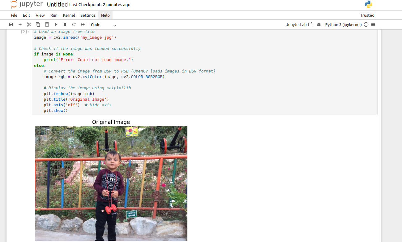
# Load an image from file
image = cv2.imread('my_image.jpg')

# Check if the image was loaded successfully
if image is None:
    print("Error: Could not load image.")
else:
    # Convert the image from BGR to RGB (OpenCV loads images in BGR format)
    image_rgb = cv2.cvtColor(image, cv2.COLOR_BGR2RGB)

    # Display the image using matplotlib
    plt.imshow(image_rgb)
    plt.title('Original Image')
    plt.axis('off')  # Hide axis
    plt.show()
Explanation:
- cv2.imread(‘my_image.jpg’): Loads the image from the file. Replace ‘my_image.jpg’ with the path to your image.
- cv2.cvtColor(image, cv2.COLOR_BGR2RGB): Converts the image from BGR (OpenCV default) to RGB for proper display with matplotlib.
- plt.imshow(image_rgb): Displays the image.
- plt.axis(‘off’): Hides the axis for a cleaner view.
Output:
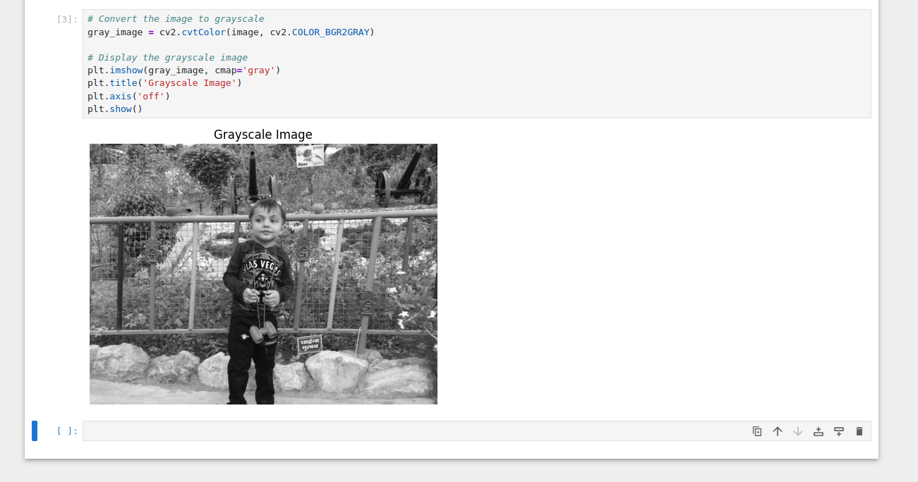
Step 5: Convert the Image to Grayscale
Convert the image to grayscale, as many image processing tasks work better on grayscale images:
# Convert the image to grayscale
gray_image = cv2.cvtColor(image, cv2.COLOR_BGR2GRAY)

# Display the grayscale image
plt.imshow(gray_image, cmap='gray')
plt.title('Grayscale Image')
plt.axis('off')
plt.show()
Explanation:
- cv2.cvtColor(image, cv2.COLOR_BGR2GRAY): Converts the image to grayscale.
- cmap=’gray’: Ensures the grayscale image is displayed correctly.
Output:
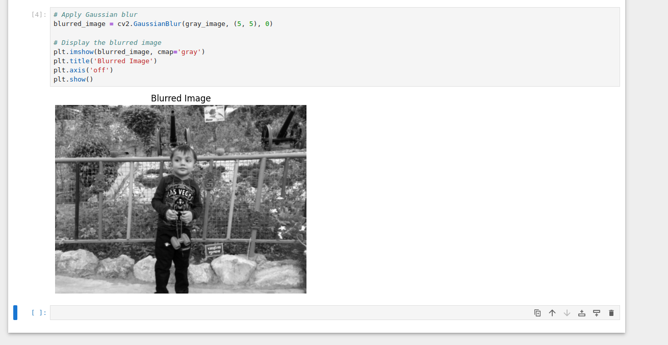
Step 6: Apply Gaussian Blur
Blurring the image helps reduce noise and improve segmentation results:
# Apply Gaussian blur
blurred_image = cv2.GaussianBlur(gray_image, (5, 5), 0)

# Display the blurred image
plt.imshow(blurred_image, cmap='gray')
plt.title('Blurred Image')
plt.axis('off')
plt.show()
Explanation:
- cv2.GaussianBlur(gray_image, (5, 5), 0): Applies Gaussian blur with a 5×5 kernel. You can adjust the kernel size for more or less blur.
Output:
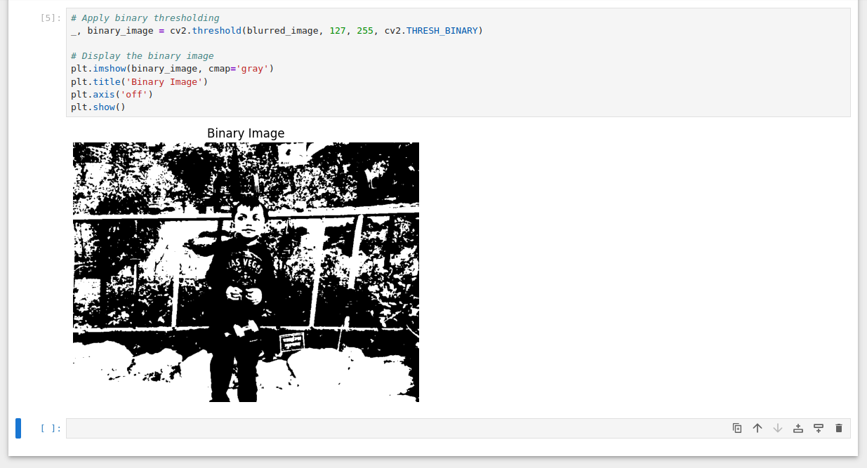
Step 7: Apply Thresholding
Thresholding is a simple way to segment an image into foreground and background:
# Apply binary thresholding
_, binary_image = cv2.threshold(blurred_image, 127, 255, cv2.THRESH_BINARY)

# Display the binary image
plt.imshow(binary_image, cmap='gray')
plt.title('Binary Image')
plt.axis('off')
plt.show()
Explanation:
- cv2.threshold(blurred_image, 127, 255, cv2.THRESH_BINARY): Applies binary thresholding. Pixels with intensity > 127 are set to 255 (white), and others are set to 0 (black).
Output:
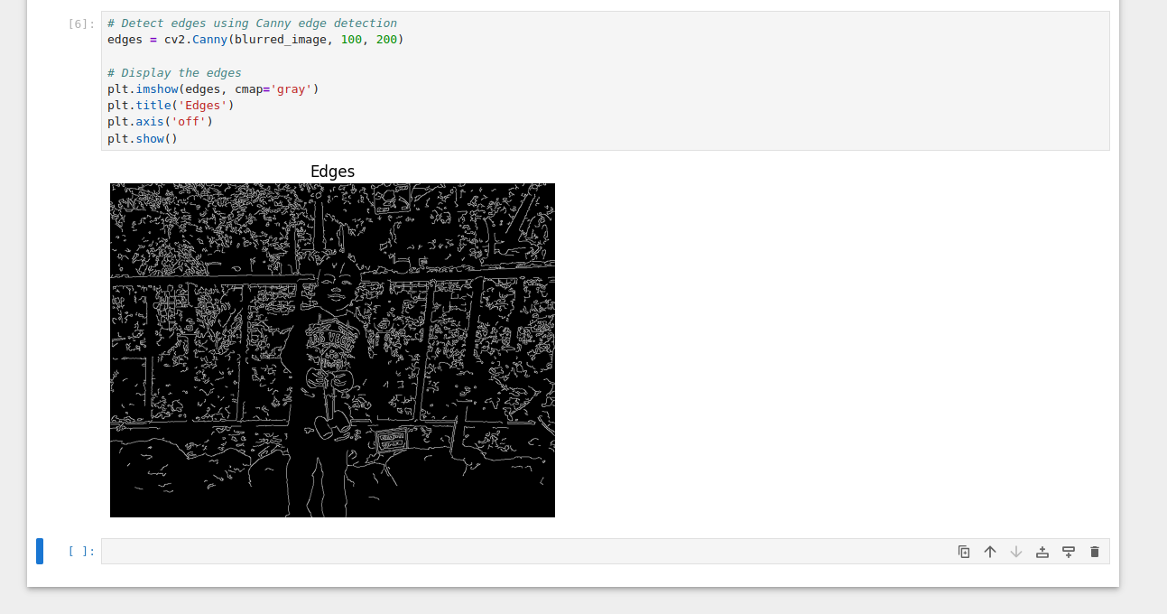
Step 8: Detect Edges Using Canny Edge Detection
Edge detection is another common technique for image segmentation:
# Detect edges using Canny edge detection
edges = cv2.Canny(blurred_image, 100, 200)

# Display the edges
plt.imshow(edges, cmap='gray')
plt.title('Edges')
plt.axis('off')
plt.show()
Explanation:
- cv2.Canny(blurred_image, 100, 200): Detects edges using the Canny algorithm. The thresholds 100 and 200 control the sensitivity of edge detection.
Output:
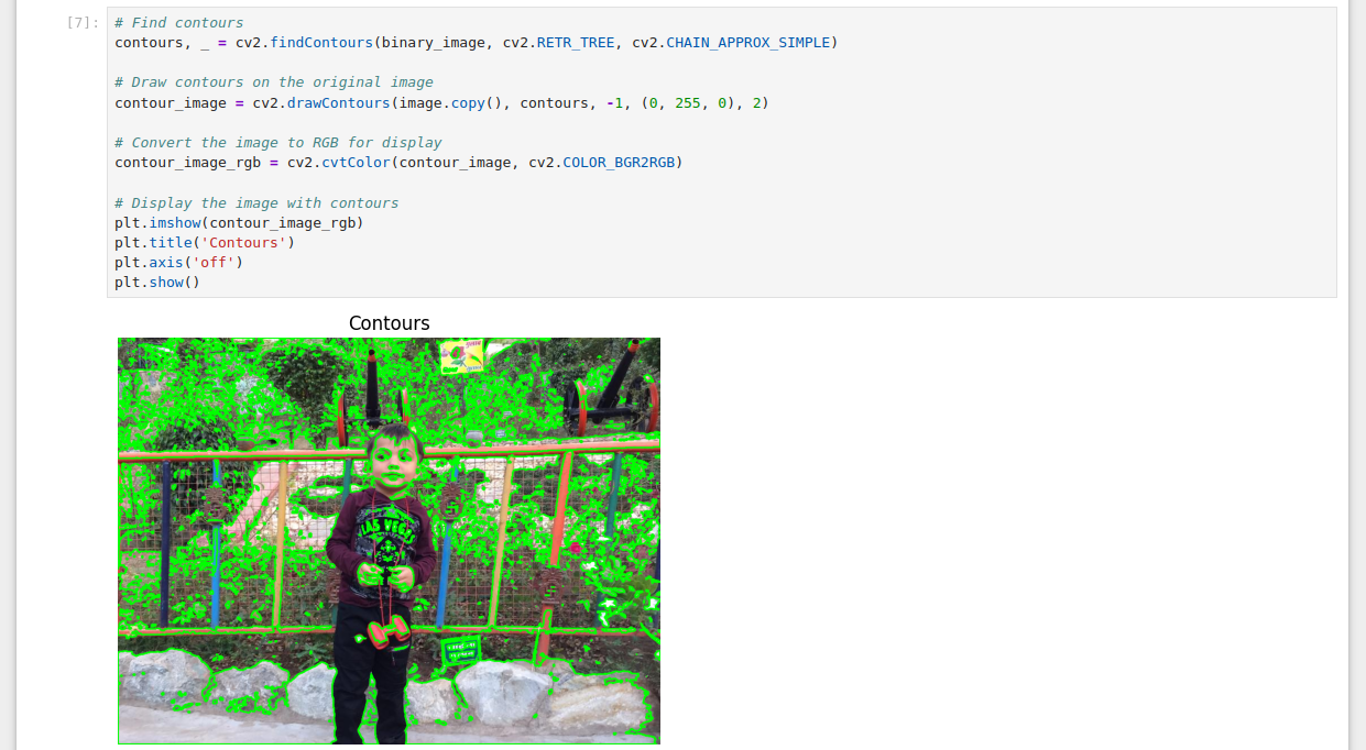
Step 9: Find Contours
Contours are useful for identifying objects in an image:
# Find contours
contours, _ = cv2.findContours(binary_image, cv2.RETR_TREE, cv2.CHAIN_APPROX_SIMPLE)

# Draw contours on the original image
contour_image = cv2.drawContours(image.copy(), contours, -1, (0, 255, 0), 2)

# Convert the image to RGB for display
contour_image_rgb = cv2.cvtColor(contour_image, cv2.COLOR_BGR2RGB)

# Display the image with contours
plt.imshow(contour_image_rgb)
plt.title('Contours')
plt.axis('off')
plt.show()
Explanation:
- cv2.findContours(binary_image, cv2.RETR_TREE, cv2.CHAIN_APPROX_SIMPLE): Finds contours in the binary image.
- cv2.drawContours(image.copy(), contours, -1, (0, 255, 0), 2): Draws contours on a copy of the original image. The color (0, 255, 0) is green, and 2 is the thickness of the contour lines.
Output:
Step 10: Save the Final Output
Finally, save the image with contours to a file:
# Save the image with contours
cv2.imwrite('output_image.jpg', cv2.cvtColor(contour_image_rgb, cv2.COLOR_RGB2BGR))
print("Output image saved as 'output_image.jpg'")
Explanation:
- cv2.imwrite(‘output_image.jpg’, contour_image_rgb): Saves the image with contours to a file.
Conclusion
By following these steps in a Jupyter Notebook you can build a simple image segmentation pipeline using OpenCV. The notebook environment allows you to visualize each step of the process, so you can understand and debug it better. You can further extend this pipeline with more advanced techniques like semantic segmentation or deep learning based approaches.
* This post is for informational purposes only and does not constitute professional, legal, financial, or technical advice. Each situation is unique and may require guidance from a qualified professional.
Readers should conduct their own due diligence before making any decisions.