Machine learning (ML) has become a tool for solving many problems, from predicting house prices to recommending movies. Among the many libraries for ML in Python, Scikit-learn is one of the most popular. Scikit-learn is a robust and easy to use framework for implementing and testing machine learning algorithms. It includes tools for data preprocessing, dataset splitting, model training and evaluation.
In this tutorial, you’ll learn how to build your first machine learning model using Scikit-learn on Atlantic.Net Cloud GPU.
Prerequisites
- An Ubuntu 22.04 Cloud GPU Server.
- CUDA Toolkit and cuDNN Installed.
- A root or sudo privileges.
Step 1: Setting Up the Environment
Before we begin coding, you need to install the required Python libraries. Open a terminal and execute the following commands:
pip install scikit-learn pandas seabornNext, install the Jupyter Notebook.
pip install notebookNext, launch a Jupyter Notebook using the below command.
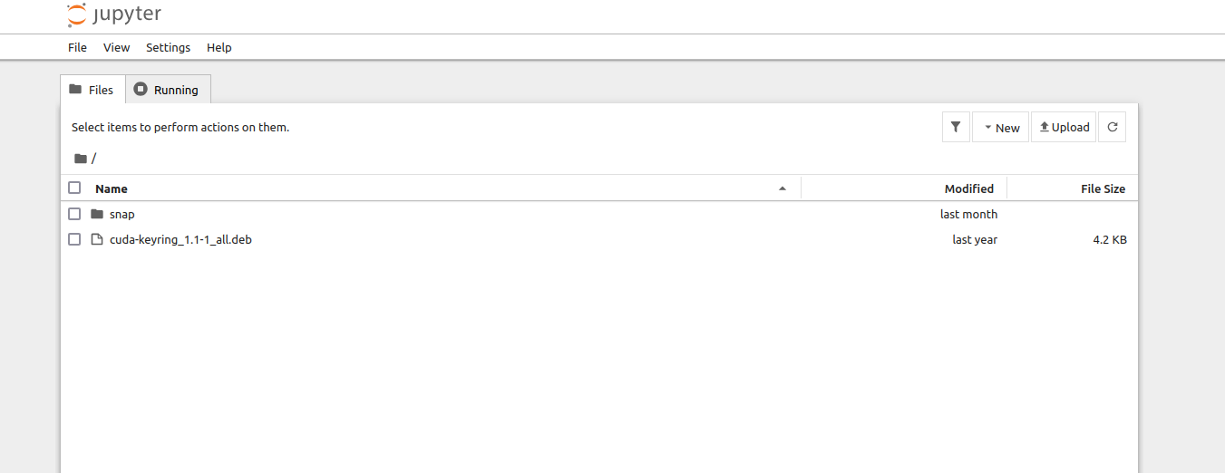
jupyter notebook --no-browser --port=8888 --ip=your-server-ip --allow-rootAfter running the jupyter notebook command, you will see a URL in your terminal.
Open your web browser and use this URL to access the Jupyter Notebook.
Note: If you cannot access the Notebook, check to see if your Firewall is blocking traffic.
Click on File > New > Notebook. You will be asked to select the Kernel.
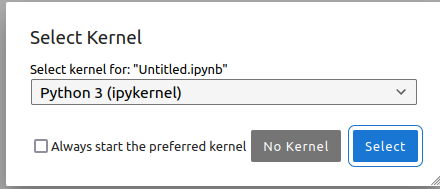
Select the “Python (GPU)” kernel and click Select to create a new notebook.
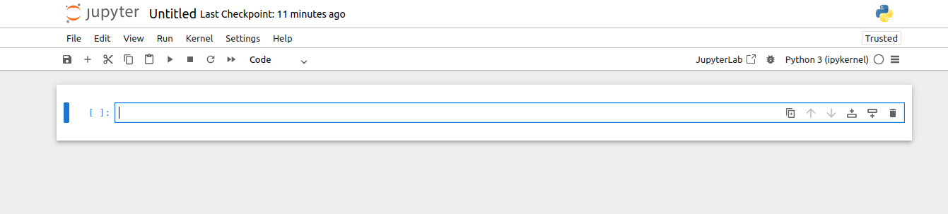
Jupyter Notebook allows you to write and execute Python code in a browser-based interface interactively. We will perform remaining steps in Jupyter Notebook.
Step 2: Import Libraries and Prepare the Dataset
Once the environment is set up, start by importing the necessary libraries and creating a small dataset.
import numpy as np
import pandas as pd
from sklearn.model_selection import train_test_split
from sklearn.linear_model import LinearRegression
from sklearn.metrics import mean_squared_error, r2_score
import seaborn as sns
import matplotlib.pyplot as plt
# Example dataset
data = pd.DataFrame({
'Feature1': [1, 2, 3, 4, 5],
'Feature2': [2, 4, 6, 8, 10],
'PRICE': [3, 6, 9, 12, 15]
})
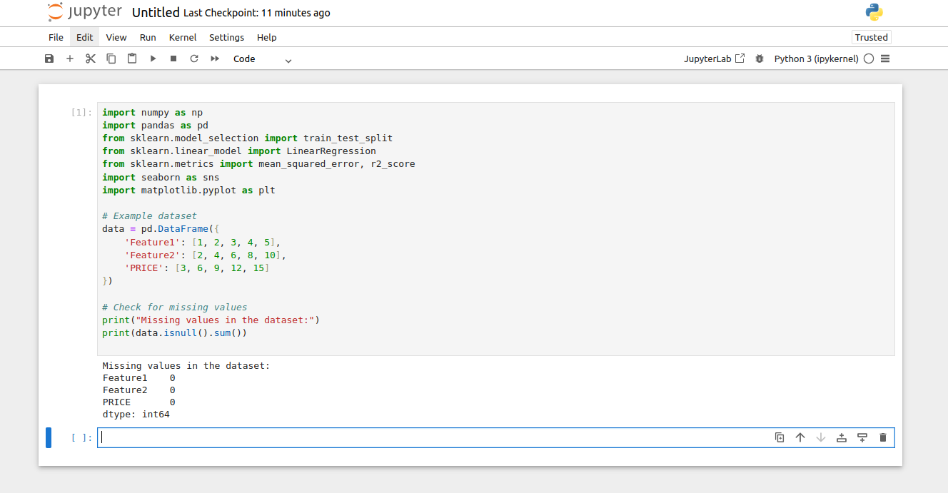
# Check for missing values
print("Missing values in the dataset:")
print(data.isnull().sum())In this code:
- We imported essential libraries for machine learning (sklearn), data handling (pandas), and visualization (seaborn, matplotlib).
- The data DataFrame is a simple dataset with two features (Feature1, Feature2) and a target variable (PRICE) to illustrate regression.
- Missing values can create issues during model training, so we check them using isnull().sum().
Step 3: Visualize Data Relationships
Visualization provides insights into how features are related to each other and the target variable.
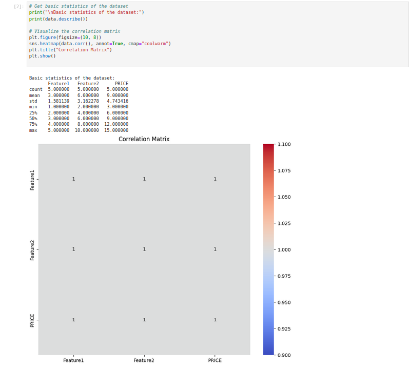
# Get basic statistics of the dataset
print("\nBasic statistics of the dataset:")
print(data.describe())

# Visualize the correlation matrix
plt.figure(figsize=(10, 8))
sns.heatmap(data.corr(), annot=True, cmap="coolwarm")
plt.title("Correlation Matrix")
plt.show()
Here:
- The describe() function provides an overview of the dataset, such as mean, min, and max values, which helps us understand its range and variability.
- The correlation matrix reveals the strength of relationships between variables.
- Values close to 1 or -1 indicate strong positive or negative correlations, while values close to 0 show weak or no correlation.
Step 4: Define Features and Split Data
Machine learning models require separating features (independent variables) from the target (dependent variable). Then, we split the data into training and testing sets.
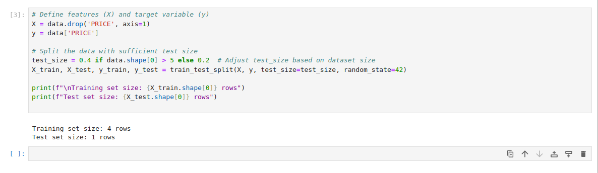
# Define features (X) and target variable (y)
X = data.drop('PRICE', axis=1)
y = data['PRICE']

# Split the data with sufficient test size
test_size = 0.4 if data.shape[0] > 5 else 0.2  # Adjust test_size based on dataset size
X_train, X_test, y_train, y_test = train_test_split(X, y, test_size=test_size, random_state=42)

print(f"\nTraining set size: {X_train.shape[0]} rows")
print(f"Test set size: {X_test.shape[0]} rows")
Here:
- The feature set (X) is created by dropping the PRICE column, and y stores the target variable.
- Using train_test_split, we divide the data into training (to build the model) and testing (to evaluate it). Adjusting test_size ensures a sufficient split based on dataset size.
Step 5: Train the Model
Fit a linear regression model to the training data. We also use the trained model to predict the target variable for the test set.
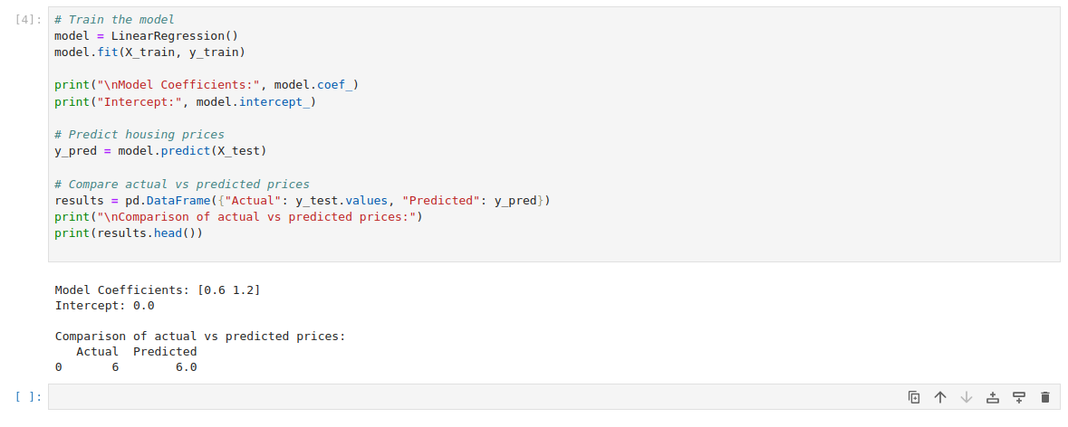
# Train the model
model = LinearRegression()
model.fit(X_train, y_train)

print("\nModel Coefficients:", model.coef_)
print("Intercept:", model.intercept_)

# Predict housing prices
y_pred = model.predict(X_test)

# Compare actual vs predicted prices
results = pd.DataFrame({"Actual": y_test.values, "Predicted": y_pred})
print("\nComparison of actual vs predicted prices:")
print(results.head())
Here:
- The LinearRegression model learns a linear relationship between X_train and y_train.
- The coef_ and intercept_ values represent the slope and intercept of the regression line, which the model uses for predictions.
- The predict method generates predictions for X_test using the trained model.
- A DataFrame (results) compares actual and predicted values to help visualize the model’s accuracy.
Step 6: Evaluate the Model
Evaluate the model’s performance using metrics such as Mean Squared Error (MSE) and R-squared. Then, create a scatter plot to visualize how closely the predicted values align with the actual values.
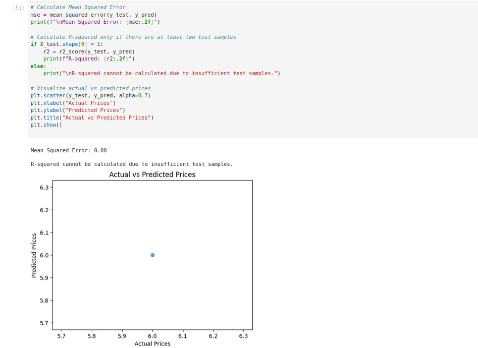
# Calculate Mean Squared Error
mse = mean_squared_error(y_test, y_pred)
print(f"\nMean Squared Error: {mse:.2f}")

# Calculate R-squared only if there are at least two test samples
if X_test.shape[0] > 1:
    r2 = r2_score(y_test, y_pred)
    print(f"R-squared: {r2:.2f}")
else:
    print("\nR-squared cannot be calculated due to insufficient test samples.")

# Visualize actual vs predicted prices
plt.scatter(y_test, y_pred, alpha=0.7)
plt.xlabel("Actual Prices")
plt.ylabel("Predicted Prices")
plt.title("Actual vs Predicted Prices")
plt.show()
Here:
- MSE quantifies the average squared error between actual and predicted values, where lower values indicate better performance.
- R-squared explains how well the features predict the target variable, with values closer to 1 indicating a better fit.
Conclusion
Congratulations! You’ve completed your first machine learning model with Scikit-learn in Jupyter Notebook. This hands on approach is perfect for learning the basics of ML and Jupyter’s interactivity makes it easy to test and visualize. Now go experiment with larger datasets, more features and different algorithms.
* This post is for informational purposes only and does not constitute professional, legal, financial, or technical advice. Each situation is unique and may require guidance from a qualified professional.
Readers should conduct their own due diligence before making any decisions.