Table of Contents
- Prerequisites
- Step 1: Install Required Software
- Step 2: Create an In-Memory Dataset
- Step 3: Define a Machine Learning Pipeline
- Step 4: Define Hyperparameter Grid
- Step 5: Initialize GridSearchCV
- Step 6: Fit the Model
- Step 7: Running the Code in a Jupyter Notebook
- Step 8: Monitor GPU Usage
- Step 9: Save and Download Results
- Conclusion
Hyperparameter tuning is an important step in improving the performance of machine learning models. By tuning the hyperparameters, we can boost the predictive power of the models. One way of hyperparameter tuning is GridSearchCV, which exhaustively searches through a grid of hyperparameter combinations.
Due to computational constraints, running GridSearchCV on a local machine is impractical when working with large datasets or complex models. Using a cloud GPU can speed up this process.
In this tutorial, we will go through the steps to perform hyperparameter tuning with GridSearchCV on a cloud GPU.
Prerequisites
- An Ubuntu 22.04 Cloud GPU Server.
- CUDA Toolkit, cuDNN Installed.
- Jupyter Notebook is installed and running.
- A root or sudo privileges.
Step 1: Install Required Software
Before starting, you will need to install the necessary dependencies, including drivers for GPU acceleration and libraries for machine learning tasks.
pip install numpy pandas scikit-learn matplotlibStep 2: Create an In-Memory Dataset
We will first create a small in-memory dataset using Python’s pandas library. This dataset will serve as input for the model.
import pandas as pd
from sklearn.pipeline import Pipeline
from sklearn.preprocessing import StandardScaler
from sklearn.ensemble import RandomForestClassifier
from sklearn.model_selection import GridSearchCV

# Create an in-memory dataset
data_dict = {
    'feature1': [1, 4, 7, 2, 9],
    'feature2': [2, 5, 8, 5, 3],
    'feature3': [3, 6, 9, 3, 5],
    'target':    [0, 1, 0, 1, 0]
}

# Convert dictionary to DataFrame
data = pd.DataFrame(data_dict)

# 2. Split into features (X) and labels (y)
X = data.drop("target", axis=1)
y = data["target"]
Here, the dataset contains three features and a target variable. The X variable holds the features, and y holds the target.
Step 3: Define a Machine Learning Pipeline
A pipeline helps streamline preprocessing and model training steps. Here, we scale the features and train a random forest classifier:
pipeline = Pipeline([
    ('scaler', StandardScaler()),
    ('classifier', RandomForestClassifier(random_state=42))
])
The pipeline first applies feature scaling using StandardScaler, which normalizes the data. Then, it trains a RandomForestClassifier on the scaled features.
Step 4: Define Hyperparameter Grid
Hyperparameters are configurations external to the model, and tuning them can significantly affect performance. Define a grid of values to search:
param_grid = {
    'classifier__n_estimators': [100, 200, 300],
    'classifier__max_depth': [10, 20, 30],
    'classifier__min_samples_split': [2, 5, 10]
}
Here, we tune three parameters of the RandomForestClassifier: the number of estimators, maximum depth, and minimum samples required to split a node.
Step 5: Initialize GridSearchCV
GridSearchCV performs an exhaustive search over the parameter grid to find the best combination:
grid_search = GridSearchCV(
    estimator=pipeline,
    param_grid=param_grid,
    scoring='accuracy',
    cv=2,    # <-- Reduced from 5 to 2
    n_jobs=-1
)
This setup optimizes the accuracy score, uses 2-fold cross-validation, and parallelizes computations for efficiency.
Step 6: Fit the Model
Train the model using the defined parameter grid:
grid_search.fit(X, y)

print("Best Parameters:", grid_search.best_params_)
print("Best Score:", grid_search.best_score_)
The fit method evaluates all parameter combinations, and best_params_ shows the optimal hyperparameters. best_score_ displays the highest cross-validated accuracy.
Step 7: Running the Code in a Jupyter Notebook
Create a new notebook from the Jupyter Notebook dashboard, combine all code and paste them into the notebook cell, then run the notebook to observe the outputs.
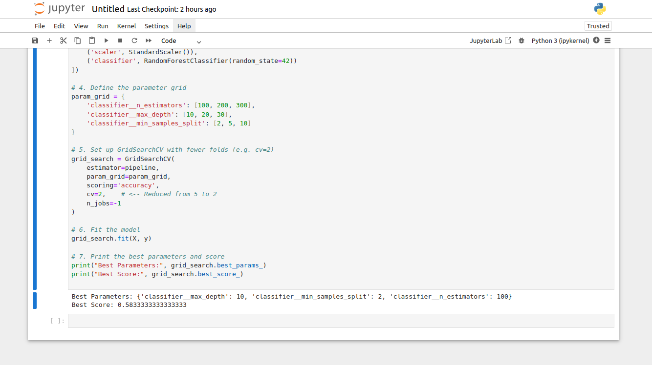
The above image displays the best hyperparameter values ({‘classifier__max_depth’: 10, ‘classifier__min_samples_split’: 2, ‘classifier__n_estimators’: 100}) and the corresponding accuracy score (0.583333…).
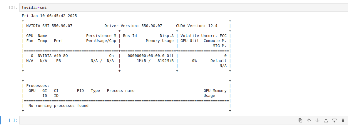
Step 8: Monitor GPU Usage
To ensure the GPU is utilized efficiently, monitor its usage with:
!nvidia-smiThis command shows GPU utilization, memory usage, and active processes.
Step 9: Save and Download Results
Save the best-performing model to a file for future use.
import joblib
joblib.dump(grid_search.best_estimator_, "best_model.pkl")
This creates a portable file containing the trained model, which can be loaded later for inference. You can download this model using SCP or FTP method.
Conclusion
Performing hyperparameter tuning with GridSearchCV on a cloud GPU is much faster for large datasets or complex models. Follow this guide to set up and execute hyperparameter optimization in the cloud. Each step, from preparing the dataset to saving the results, is designed to be efficient and accurate. With the right setup, you will get the best out of your machine learning model.