Table of Contents
- Prerequisites
- Step 1: Install Required Libraries
- Step 2: Download and Extract the Dataset
- Step 3: Dataset Preparation
- Step 4: Load and Modify the Pretrained Model
- Step 5: Define Training Setup
- Step 6: Train the Model
- Step 7: Validate the Model
- Step 8: Verify the Model with a Sample Image
- Step 9: Run the Code in Jupyter Notebook
- Conclusion
Deep learning has changed how we approach image classification tasks, but training a deep neural network from scratch requires a huge amount of labeled data and computational resources. This is where transfer learning comes in. Transfer learning uses pre-trained models such as ResNet-5,0, which have already learned general features from large datasets like ImageNet. These models can be fine-tuned for a specific task, reducing training time and the need for large datasets.
In this tutorial, we will show you how to implement transfer learning using PyTorch to classify flowers from the Flowers Dataset.
Prerequisites
- An Ubuntu 22.04 Cloud GPU Server.
- CUDA Toolkit, cuDNN Installed.
- Jupyter Notebook is installed and running.
- A root or sudo privileges.
Step 1: Install Required Libraries
Before starting, you will need to install PyTorch with GPU support on your server. You can install them with the following command.
pip install torch torchvision torchaudio --index-url https://download.pytorch.org/whl/cu124Step 2: Download and Extract the Dataset
To begin, we’ll use the Flowers dataset provided by TensorFlow. It contains labeled images of five flower classes: daisy, dandelion, roses, sunflowers, and tulips.
# Import necessary libraries
import os
import random
import torch
import torch.nn as nn
import torch.optim as optim
import matplotlib.pyplot as plt
from torchvision import datasets, transforms, models
from PIL import Image

# Check for GPU availability
device = torch.device('cuda' if torch.cuda.is_available() else 'cpu')

#Download and Extract Dataset
# Download and extract the dataset
if not os.path.exists('dataset/flower_photos'):
    os.system('wget http://download.tensorflow.org/example_images/flower_photos.tgz')
    os.system('mkdir -p dataset')
    os.system('tar -xzf flower_photos.tgz -C dataset')
Explanation:
- The code checks if the dataset exists locally.
- If not, it downloads the dataset (flower_photos.tgz) and extracts it into the dataset/flower_photos directory.
Step 3: Dataset Preparation
We prepare the dataset for training and validation. Images are resized to 224×224 pixels and converted to PyTorch tensors. The dataset is split into 80% training and 20% validation.
# Define transformations for preprocessing
transform = transforms.Compose([
    transforms.Resize((224, 224)),  # Resize images to 224x224 pixels
    transforms.ToTensor(),          # Convert images to PyTorch tensors
])

# Load the dataset and split into training and validation sets
dataset_path = 'dataset/flower_photos'
train_dataset = datasets.ImageFolder(dataset_path, transform=transform)
val_split = int(len(train_dataset) * 0.2)  # Use 20% for validation
train_split = len(train_dataset) - val_split

train_dataset, val_dataset = torch.utils.data.random_split(
    train_dataset, [train_split, val_split]
)

# Create DataLoaders
train_loader = torch.utils.data.DataLoader(train_dataset, batch_size=32, shuffle=True)
val_loader = torch.utils.data.DataLoader(val_dataset, batch_size=32, shuffle=False)

# Print dataset statistics
print(f"Classes: {train_dataset.dataset.classes}")  # ['daisy', 'dandelion', 'roses', 'sunflowers', 'tulips']
print(f"Number of training samples: {len(train_dataset)}")
print(f"Number of validation samples: {len(val_dataset)}")
Explanation:
- Transformations: Resize images to 224×224 to match the input size for ResNet and convert them into tensors.
- Data Splitting: The dataset is split into training (80%) and validation (20%) subsets for model training and evaluation.
- Data Loaders: These enable efficient batch processing during training and validation.
Step 4: Load and Modify the Pretrained Model
PyTorch provides a variety of pre-trained models via torch-vision models. Here, we use ResNet-50 and modify its final layer to classify five flower types.
# Load pretrained ResNet-50 model
model = models.resnet50(pretrained=True)

# Freeze pretrained layers
for param in model.parameters():
    param.requires_grad = False

# Replace the final classification layer to match the number of classes
num_classes = len(train_dataset.dataset.classes)
model.fc = nn.Linear(model.fc.in_features, num_classes)
model = model.to(device)
Explanation:
- Freezing Layers: Prevents updates to the pretrained layers, preserving their learned features.
- Final Layer Replacement: The original 1000-class output layer is replaced with a new layer for five flower classes.
Step 5: Define Training Setup
We define the loss function and optimizer required for training.
# Loss function and optimizer
criterion = nn.CrossEntropyLoss()
optimizer = optim.Adam(model.fc.parameters(), lr=0.001)
Explanation:
- Loss Function: CrossEntropyLoss is suitable for multi-class classification problems.
- Optimizer: Adam optimizer updates only the parameters of the newly added final layer.
Step 6: Train the Model
Train the model over multiple epochs, calculating the loss for each batch and updating weights accordingly.
epochs = 5
for epoch in range(epochs):
    model.train()
    running_loss = 0.0

    for inputs, labels in train_loader:
        inputs, labels = inputs.to(device), labels.to(device)

        optimizer.zero_grad()
        outputs = model(inputs)
        loss = criterion(outputs, labels)
        loss.backward()
        optimizer.step()

        running_loss += loss.item()

    print(f"Epoch {epoch+1}/{epochs}, Loss: {running_loss/len(train_loader)}")
Explanation:
- Training Mode: The model is set to training mode using model.train().
- Batch Processing: Each batch of inputs and labels is passed through the model to calculate and backpropagate the loss.
- Loss Monitoring: Average loss per epoch is printed to track training progress.
Step 7: Validate the Model
Evaluate the model’s accuracy on the validation set.
model.eval()
correct = 0
total = 0

with torch.no_grad():
    for inputs, labels in val_loader:
        inputs, labels = inputs.to(device), labels.to(device)
        outputs = model(inputs)
        _, predicted = torch.max(outputs, 1)
        total += labels.size(0)
        correct += (predicted == labels).sum().item()

print(f'Validation Accuracy: {100 * correct / total:.2f}%')
Explanation:
- Evaluation Mode: Disables dropout and batch normalization using model.eval().
- Prediction: Compares predicted labels with actual labels to calculate accuracy.
Step 8: Verify the Model with a Sample Image
Select a random image from the dataset and visualize the model’s prediction.
# Get a random image path from one of the class directories
sample_dir = os.path.join(dataset_path, random.choice(train_dataset.dataset.classes))
sample_image_path = os.path.join(sample_dir, random.choice(os.listdir(sample_dir)))

print(f"Using sample image: {sample_image_path}")

# Load and preprocess the sample image
image = Image.open(sample_image_path)
input_tensor = transform(image).unsqueeze(0).to(device)

# Get prediction
model.eval()
with torch.no_grad():
    output = model(input_tensor)
    _, predicted = torch.max(output, 1)

# Map prediction to class name
predicted_class = train_dataset.dataset.classes[predicted.item()]
print(f"Predicted Class: {predicted_class}")

# Visualize the image with its predicted label
plt.imshow(image)
plt.title(f'Predicted: {predicted_class}')
plt.axis('off')
plt.show()
Explanation:
- Random Image Selection: Picks a random image from the dataset for testing.
- Prediction: Passes the image through the model and retrieves the predicted class.
- Visualization: Displays the image with the predicted class label.
Step 9: Run the Code in Jupyter Notebook
Create a new notebook from Jupyter Notebook, add all the code to the notebook cell, and then run the notebook.
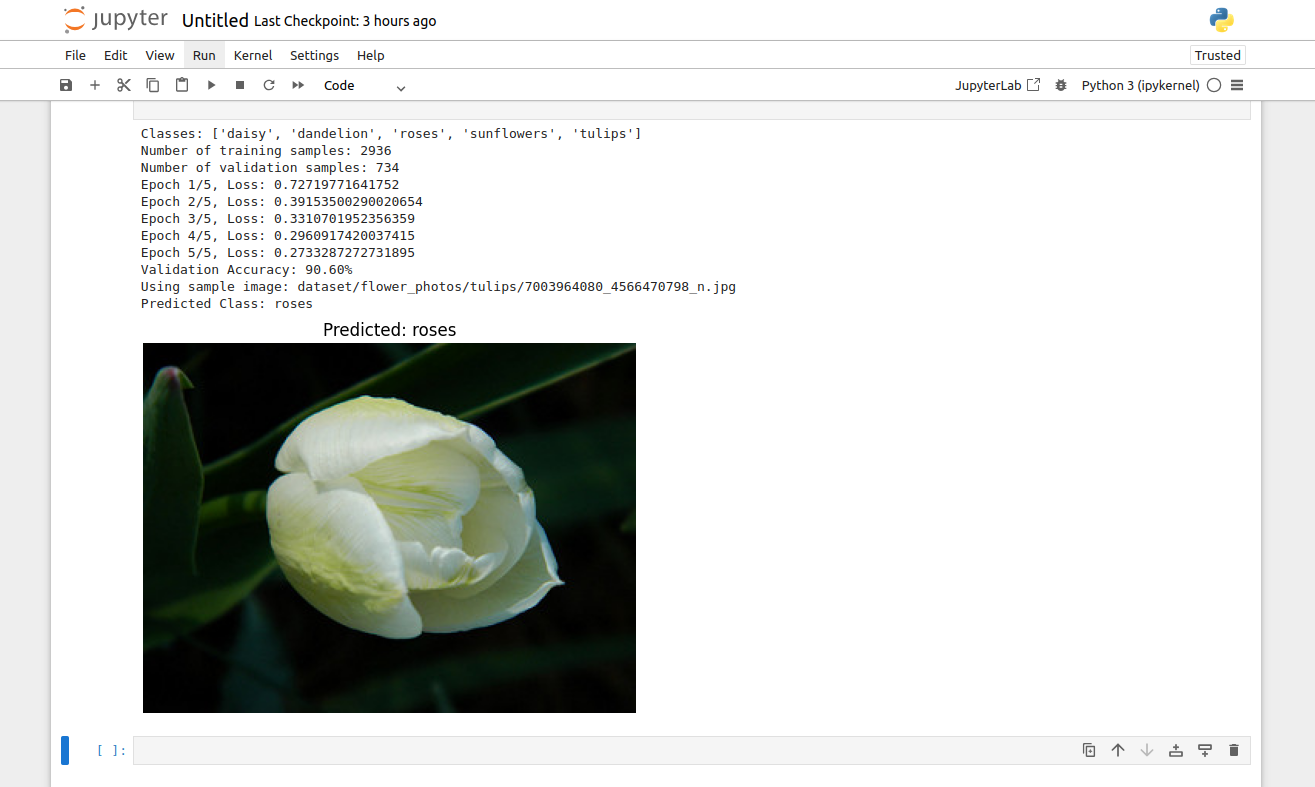
The above image demonstrates the notebook’s final output. Here, the model has been trained over five epochs, achieving a validation accuracy of 90.60%. A sample image of a flower from the validation set was randomly selected, and the model predicted its class as roses. The displayed image visually confirms the prediction, highlighting the model’s accuracy.
Conclusion
In this tutorial, we went through transfer learning with PyTorch to build robust classifiers for image classification tasks. We used the pre-trained ResNet-50 model and avoided training a model from scratch, and got high accuracy on the Flowers dataset. We went through data preparation, model fine-tuning, training, and validation, and finally, we visualized the results. You can use Atlantic.Net GPU server hosting as a platform for AI image classification and other applications!
* This post is for informational purposes only and does not constitute professional, legal, financial, or technical advice. Each situation is unique and may require guidance from a qualified professional.
Readers should conduct their own due diligence before making any decisions.