Table of Contents
- Prerequisites
- Step 1: Installing Necessary Libraries
- Step 2: Load the Dataset
- Step 3: Train-Test Split
- Step 4: Train a Random Forest Model
- Step 5: Explain Predictions with SHAP
- Step 6: Analyze SHAP Values
- Step 7: Explain Predictions with LIME
- Step 8: Analyze a Specific Instance
- Step 9: Running the Code in a Jupyter Notebook
- Conclusion
In machine learning, having a good model is only half the battle. Understanding how the model makes predictions is just as important especially when working with complex datasets or making decisions that impact business, healthcare or finance. This is where model interpretability comes in. Techniques like SHAP (SHapley Additive exPlanations) and LIME (Local Interpretable Model-agnostic Explanations) are great tools to explain the inner workings of machine learning models.
This article will walk you through the visualization of machine learning models using SHAP and LIME, with a hands-on example. We will use the Iris dataset and a Random Forest classifier to demonstrate and run the model in Jupyter Notebook.
Prerequisites
- An Ubuntu 22.04 Cloud GPU Server.
- CUDA Toolkit, cuDNN Installed.
- Jupyter Notebook is installed and running.
- A root or sudo privileges.
Step 1: Installing Necessary Libraries
Before diving into the implementation, ensure you have the required libraries installed in your environment. Use the following command to install them:
pip install pandas ipywidgets numpy matplotlib scikit-learn shap lime Step 2: Load the Dataset
We’ll use the Iris dataset, a classic dataset in machine learning, to train a Random Forest classifier. The dataset contains information about different flower species and their features such as sepal length, sepal width, petal length, and petal width.
import pandas as pd
import shap
from sklearn.datasets import load_iris
from sklearn.ensemble import RandomForestClassifier
from sklearn.model_selection import train_test_split
from lime.lime_tabular import LimeTabularExplainer

data = load_iris()
X = pd.DataFrame(data.data, columns=data.feature_names)
y = data.target
Here:
- X contains the feature values.
- y contains the target class labels for each flower species.
Step 3: Train-Test Split
We split the dataset into training and testing sets to evaluate the model’s performance. This ensures that the model is trained on one part of the data and tested on another.
X_train, X_test, y_train, y_test = train_test_split(
    X, y, test_size=0.2, random_state=42
)
Here:
- test_size=0.2: Reserves 20% of the data for testing.
- random_state=42: Ensures reproducibility of the split.
Step 4: Train a Random Forest Model
A random forest is a robust ensemble learning method that operates by constructing multiple decision trees and outputting the class, which is the mode of the classes of the individual trees. We’ll train this model using the training set.
model = RandomForestClassifier(random_state=42)
model.fit(X_train, y_train)
The trained model can now be used for predictions and analysis.
Step 5: Explain Predictions with SHAP
SHAP provides a unified measure of feature importance by attributing a prediction’s outcome to individual features. It uses Shapley values from cooperative game theory to explain predictions.
explainer = shap.Explainer(model, X_train)
shap_values = explainer(X_test, check_additivity=False)

print("shap_values.values.shape:", shap_values.values.shape)
# Typically (n_samples, n_classes, n_features) = (30, 3, 4) for Iris
print("X_test.shape:", X_test.shape)
Here:
- check_additivity=False: Disables additivity checks, which is often necessary for ensemble models like Random Forests.
- shap_values: Contains SHAP values for all features in the test set.
Step 6: Analyze SHAP Values
The shap_values object helps us understand how each feature contributes to the model’s predictions. We can visualize these contributions globally and locally.
num_classes = shap_values.values.shape[1]
for class_idx in range(num_classes):
    # Extract Explanation object for this class only
    shap_values_class = shap_values[..., class_idx]
    print(f"\n--- Beeswarm for class {class_idx} ---")
    shap.plots.beeswarm(shap_values_class)
This visualization highlights the most influential features for each class, providing insights into the model’s decision-making process.
Step 7: Explain Predictions with LIME
LIME focuses on explaining individual predictions by approximating the model locally with an interpretable surrogate model. This makes it particularly useful for understanding specific predictions.
lime_explainer = LimeTabularExplainer(
    training_data=X_train.values,
    feature_names=X_train.columns,
    class_names=data.target_names,
    mode="classification"
)
Here:
- feature_names: Names of the features in the dataset.
- class_names: Target class labels (e.g., species of flowers)
Step 8: Analyze a Specific Instance
We’ll analyze the model’s prediction for a specific test instance.
instance = X_test.iloc[0].values
lime_exp = lime_explainer.explain_instance(
    instance,
    model.predict_proba,
    num_features=4
)

lime_exp.show_in_notebook()
lime_exp.as_pyplot_figure()
The visualization provides a breakdown of the features that contribute the most to the prediction for the selected instance.
Step 9: Running the Code in a Jupyter Notebook
Create a new notebook from the Jupyter Notebook dashboard, combine all code snippets and paste them into the notebook cell, and run the notebook to observe the outputs.
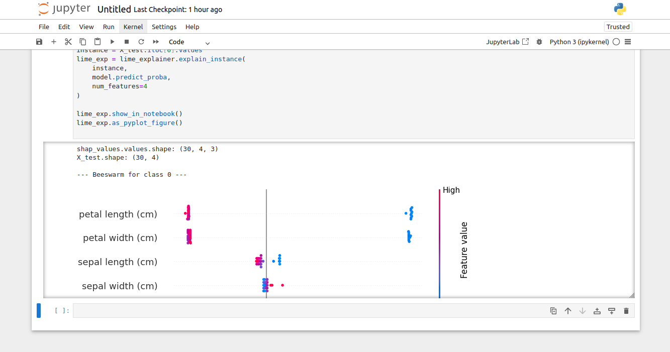
In the above result, the beeswarm plot illustrates the global importance of features, while the LIME explanation highlights the local contribution of features to an individual prediction.
Conclusion
Model interpretability is key to responsible AI. Tools like SHAP and LIME make it easier to explain predictions and trust machine learning models. In this tutorial we used the Iris dataset and a Random Forest classifier to show you how to use these tools. Start using these today on GPU hosting from Atlantic.Net to get more insights and make better decisions.
* This post is for informational purposes only and does not constitute professional, legal, financial, or technical advice. Each situation is unique and may require guidance from a qualified professional.
Readers should conduct their own due diligence before making any decisions.